Full code on Github: https://github.com/wiwa/blog-code/
Hi Link to heading
Recently, I finished a batch at the Recurse Center… is what I would have said if this post were written when I intended to write it (i.e. 3 months ago). My project there focused on a questionable application of CUDA (mostly irrelevant to this post), but it got me thinking more about other GPU-friendly algorithms.
Instead of my Recurse project (which I hope to write about in a later post), I want to simply begin writing about technical stuff I’ve played around with. Today will be about a high-level overview of a particular kind of parallel sorting algorithm called bitonic sort . I’ll go over the context behind around algorithm, a few basics of SIMD programming, a CUDA implementation, and how a small optimization grants it a +30% performance uplift. We’ll be using a SIMD-like operation (a CUDA instruction called __shfl_sync) to quickly sort 32-element “vectors”.
What is a Bitonic Sort? Link to heading
But what does the word “bitonic” even mean? This was my first question when I happened on the algo. A monotonic sequence is one whose elements are all non-decreasing or non-increasing (i.e. sorted sequences like [1,2,3,4] or [4,3,2,1]). A bitonic sequence is a sequence formed by a concatenation of two monotonic sequences, e.g. [1,3,5,4,3,2,1].
Bitonic sort is a species of sorting network, a popular family of fast, parallel (comparison) sorting algorithms. Bitonic sort, for example, can sort in O(log^2(n)) “time” (i.e. “parallel depth”/“delay”/“wall time”).
How is this possible when it’s proven that a comparison-based sort requires O(n*log(n)) time? Because that’s the runtime requirement for a sequential algorithm – specifically, the “work” needed. Bitonic sort requires O(n*log^2(n)) parallel work (total number of comparisons, or “cpu time”) which can be completely parallelized across n processors.
Usually, CS majors only care about the big-O of sorts, but constants also matter in the real world. Thankfully, bitonic sort seems to incur small constants and offers good cache locality.
Sorting networks are typically represented like a circuit with a series of parallel swaps (predicated, of course, upon a partial order). Since they are (virtual) circuits, a sorting network operates on a specific number of elements.
Here’s an example of a (“non-alternating”) bitonic sort on 16 elements:
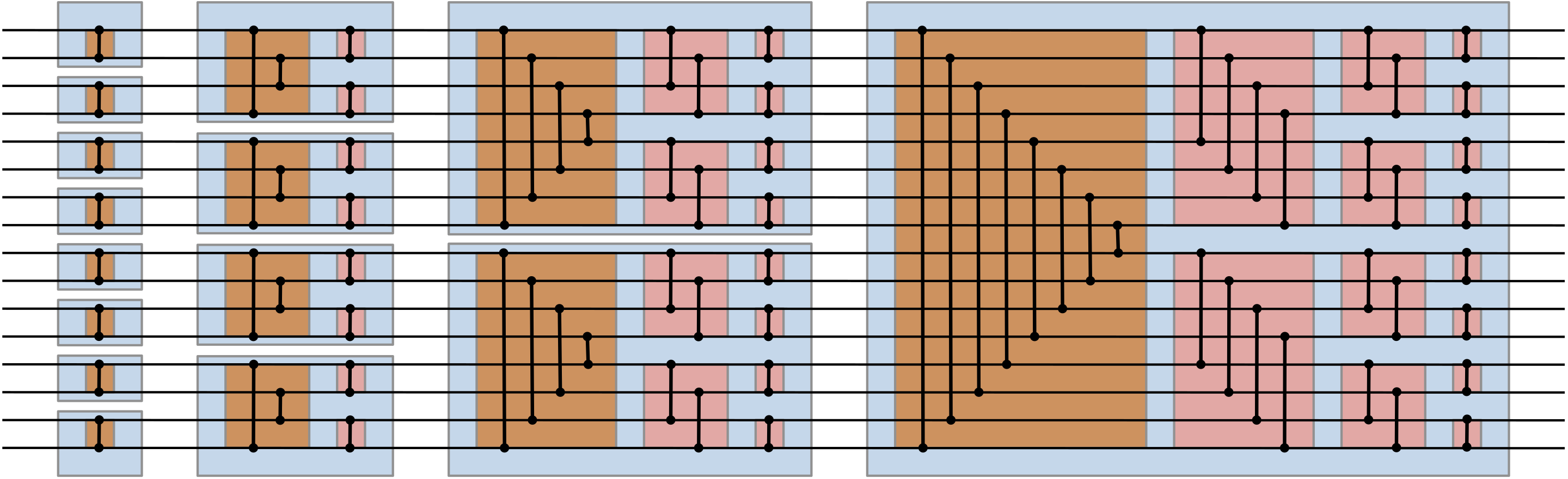
The types of bitonic sequences we’ll focus on will be made up of two monotonic sequences of equal length, e.g. if the first half is monotonically increasing, then the second half is deceasing. Implicitly, this means our sorting algorithm will only work on sequences whose size is a power of 2, at least naively. However, we can of course just pad any input with minimal/maximal values.
Sorting and SIMD Link to heading
In reality, sorting performance is more important with a growing number of elements. How can we use a fast-but-small bitonic sort to speed up a general sort of a large sequence? Imagine a merge sort where, instead of recursing down to the 2-item case, we only recurse down to the 32-item case, with the bonus that this wider “base-case” can be solved faster than the naive implementation via hardware acceleration. This is where the GPU comes into play, but it should be noted that bitonic sort can also speed up sorting on CPUs, courtesy of SIMD. That being said, we won’t go into a (CPU) SIMD implementation but rather only focus on the CUDA equivalent: warp intrinsics.
SIMD programming is quite different from typical sequential logic since it executes (in parallel) the same instruction across a vector of data (i.e. across vector lanes). Although SIMD is a parallel programming model, the term is also used to refer to “vector extensions” to CPU ISAs like AVX (x86) and NEON (ARM). Vector instructions allow us to easily hardware-accelerate data-parallel algorithms like sorting networks where each element is “small”, i.e. about the size of a word (64 bits).
An example of a SIMD data-parallel algorithm would be a map, i.e. map each item, x, in each SIMD lane to a function f, producing the resultant vector of f(x)s. An example: with 128-bit SIMD, we can have a “vector” of 4 32-bit integers, e.g. [1,3,5,7], and simultaneously operate on them with a single instruction, e.g. + [1,1,1,1] -> [2,4,6,8]. Another possible operation is reduce, e.g. sum all the numbers in the vector. However, SIMD programming allows for more interesting cases as well.
Imagine we have a vector of integers, for example [0, 1, ..., n-1], and you want to reverse it in place. One way to do this is to pair up each index with its “reverse”: (0,n-1), (1,n-2), ..., and swap the items for each pair. This is called a butterfly permutation, which is a special case of the more general idea of “shuffling”, i.e. moving data between SIMD lanes.
For those new to CUDA/GPU programming, the many different threads running on a GPU are organized into many SIMD-like executions of 32 threads each, called warps. If we have 4096 threads running, that means we have have 128 warps running in parallel, each instruction of which must execute like 32-element-wide vector instructions. However, CUDA allows the programmer to write programs as if each thread in the warp were a “normal” thread irrespective of its “neighbors” in its warp, a logical execution model which is called SIMT. Yossi Kreinin wrote a great blog post about these parallel execution models: SIMD < SIMT < SMT.
For now, when I mention “SIMD”, let’s imagine we mean warp-level execution, i.e. each thread, or “lane”, executes the same instruction in lockstep with its neighbors. If AVX512 can deal with vectors of 16 INT32s, CUDA deals with vectors of 32 INT32s.
CUDA and Code Link to heading
In CUDA, we can use the __shfl_sync built-in warp-level primitive to accomplish shuffling within a warp by directly exchanging values in registers. This is in contrast to the “traditional” method of GPU inter-thread communication in which each thread must write to/read from shared memory (L1 cache)1. In practice, this offers a significant speedup2 on its own, and I’d presume it would be even more useful if another block/kernel were already utilizing shared memory bandwidth – albeit this would probably be only a small effect considering that shared memory bandwidth is upwards of 17 TBps.
Compared to traditional CPU SIMD shuffles, __shfl_sync can handle arbitrary permutations of input lanes, like the SIMD “permutevar” ops (which take an additional vector instead of an immediate value). There’s an interesting post about SIMD shuffling here.
Here’s a code snippet illustrating the shuffle (and leaving out irrelevant details):
// load data into register
u32 datum = ...;
// Loop:
// calculate the lane to compare against
u32 other_lane = ...;
// shuffle!
u32 other_datum = __shfl_sync(gpu::all_lanes, datum, other_lane);
// swap if necessary between this lane and other_lane
// such that the smaller datum is in the lower lane index
if (lane < other_lane) {
    datum = min(datum, other_datum);
} else {
    datum = max(datum, other_datum);
}
The single call to __shfl_sync saves us a read and write to shared memory, as well as a call to __syncwarp. Warp synchronization is necessary to ensure that later reads from threads in the warp will always have the latest data. Here’s the equivalent alternative code:
u32 other_datum = shared_data[other_lane];
if (lane < other_lane) {
    datum = min(datum, other_datum);
} else {
    datum = max(datum, other_datum);
}
shared_data[lane] = datum;
// Big Green says implicit warp synchronization is an antipattern
__syncwarp();
With code in hand, it’s time to run a basic performance benchmark. The data preparation is simple: a large array of random integers. The task is to sort each 32-width subrange in a simple loop, which minimizes the effect of global memory pressure. Repeatedly the __shfl_sync version was 30% faster than using shared memory.
What now? Link to heading
It’s not a new idea to use sorting networks to lift the base-case for a general GPU mergesort from sorting 2 elements (i.e. pairs) to sorting 32 elements. ModernGPU implements another type of sorting network for their pedagogical GPU mergesort. Since they only use global memory, it’s not exactly performant, but I’d presume an industrial library like Thrust would already be using warp primitives.
But then, what else can we do with a faster 32-way sort aside from accelerating the base case? When it comes to sorting, another pairwise operation (for mergesort) is the pairwise merging of sorted sublists. In fact, that’s essentially the entire premise of mergesort. Well, what if we could somehow use it to accelerate a 32-way merge? Stay tuned for (an eventual) Part Two, because even if it’s not necessarily faster, it’s quite the funny algorithm!
For another bit of CUDA and perf, I also have a previous blog post about GPU hashmaps beating Rust by 10x: https://wiwa.substack.com/p/can-we-10x-rust-hashmap-throughput
System Details Link to heading
Ryzen 7950X3D + RTX 3090 with a PCIe 4.0x16 riser cable
I’m aware that a riser cable has perf drawbacks. But… it makes my setup prettier.
Ubuntu 22.04
CUDA 12.2